BSc Nursing 3rd Year Nursing Research And Statistics Chapter 14 Statistics Question And Answers

Statistics

Question 1. Explain the uses and application of statistics in nursing.
Answer:

Statistics in Nursing Definition

• Statistics can be defined as the collection presentation and interpretation of numerical data.
• Statistics are the numerical statement of facts in any department of inquiry placed in interrelation to each other

Application of statistics in nursing.

1. To find out the growth rate, the fertility status, and the population size of the country.
2. It facilitates knowing about the health status of the community.
3. To assess the adequacy of the medical and paramedical manpower and of the health
   institutions in the country
4. To look for the differences in the magnitude of disease by person, place, and time.
5. Statistics helps in providing a better understanding and exact description of a phenomenon of nature.
6. Statistical helps in the proper and efficient planning of a statistical inquiry in any field of study.
7. Statistical help in collecting appropriate quantitative data.
8. Statistics helps in presenting complex data in a suitable tabular, diagrammatic, and graphic form for an easy and clear comprehension of the data.
9. Statistics helps in understanding the nature and pattern of variability of a phenomenon
   through quantitative observations.
10. Statistics helps in drawing valid inferences, along with a measure of their reliability about the population parameters from the sample data.

Read And Learn More: BSc Nursing 3rd Year Nursing Research And Statistics Previous year Question And Answers 

Question 2. Functions of statistics
Answer:

1. Expression of facts in numbers – One of the main functions of Statistics is to express numbers in easily understandable language and interpret the results with certainty.
2. Simple presentation – Statistics enables the presentation of complex data in a simple format in terms of aggregate, average, percentage, graphs, diagrams, etc.
3. Enlarges individual knowledge and experience – Statistics expands the horizons of individual knowledge and understanding.
4. It compares facts – It facilitates the comparison of data and identifying the interrelations
   between large sets of data for drawing suitable inferences.
5. Facilitates policy formulation – By doing analysis and interpretation of data, the precise nature of the problem can be ascertained thus assisting policy formulation.
6. It helps other scientists in testing their laws – Statistics helps other laws establish their assumptions. E.g., many laws of economics namely the law of demand, the law of supply, and Keynes’s theory of employment can be verified by Statistics.
7. It helps in forecasting – Extrapolating present data aids in forecasting likely changes that can be expected in the future.

Question 3. Explain the most commonly used measures of dispersion.
Answer:

Methods Of Dispersion Methods of studying dispersion are divided into two types:

Mathematical Methods: We can study the ’degree‘ and ’extent‘ of variation by these methods. In this category, commonly used measures of dispersion are:

1. Range
2. Quartile Deviation
3. Average Deviation
4. Standard deviation and coefficient of variation.

Measures Of Dispersion

Dispersion is another analytical method to study data.

• A main use of dispersion is to compare the amounts of spread in two (or more) data sets.
• A common technique in inferential statistics is to draw comparisons between populations by analyzing samples that come from those populations.
• Two of the most common measures of dispersion are the range and the standard deviation.

Range:

• For any set of data, the range of the set is given by the following formula:
• Range greatest value in setting least value in the set.

Range

Example:

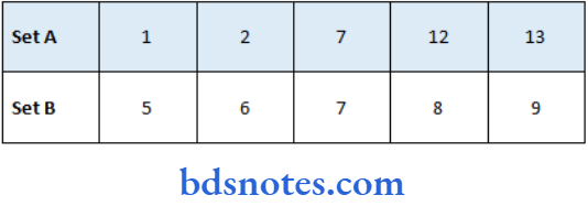
• The two sets below have the same mean and median (7). Find the range of each set.

Range of Set A: 13-1 = 12

Range of Set A: 9-5 = 4

Standard Deviation:

• One of the most useful measures of dispersion is the standard deviation.
• It is based on deviations from the mean of the data.
• Find the deviations from the mean for all data values of the samples 1, 2, 8, 11, 13.
• The mean is 7.
• To find each deviation, subtract the mean from each data value.

The sum of the deviations is always equal to zero.

Standard Deviation

Calculating the Sample Standard Deviation

\(s=\sqrt{\frac{\sum(x-\bar{x})^2}{n-1}} .\)

• The sample standard deviation is found by calculating the square root of the variance.
• The variance is found by summing the squares of the deviations and dividing that sum by (since it is a sample instead of a population).
• The sample standard deviation is denoted by the letter s.
• The standard deviation of a population is denoted by σ.

Standard Deviation

Calculating the Sample Standard Deviation

1. Calculate the mean of the numbers.
2. Find the deviations from the mean.
3. Square each deviation.
4. Sum the squared deviations.
5. Divide the sum in Step 4 by.
6. Take the square root of the quotient in Step 5.

Standard Deviation

Calculating the Sample Standard Deviation

Example:

Find the standard deviation of the sample set{1,2,8,11,13}

x = (1+2+8+11+13)/5 = 7

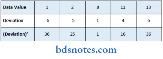
Some of the (Deviations)²2 = 36+25+1+16+36 = 114

Standard Deviation

Calculating the Sample Standard Deviation

• Some of the (Deviations)2 = 36+25+1+16+36 = 114
• Divide 114 by n- 1 with n = 5:
• Take the square root of 28.5: 5.34
• The sample standard deviation of the data is 5.34.

Question 4. Explain the uses and sources of the vital statistics.
Answer:

• Vital statistics are statistics on live births, deaths, fetal deaths, marriages, and divorces. The most common way of collecting information on these events is through civil registration an administrative system used by governments to record vital events which occur in their populations.
• Efforts to improve the quality of vital statistics will therefore be closely related to the development of civil registration systems in countries.

Vital statistics Definition:

• Vital statistics are conventionally numerical records of marriage, births, sicknesses, and deaths by which the health and growth of a community may be studied.
• Vital statistics is a part of demography and the collective study of mankind. It deals with the data related to vital events.

Uses of vital statistics:

1. Vital statistics show changing patterns in the population of a country. (medical / facilities, standard of living, etc)
2. Manufacturers plan their production by using vital statistics. (food, clothing, etc.)
3. Birth and death certificates are needed in many circumstances.
4. Accurately registered and systematically collected vital statistics can be used to check up the accuracy of data provided by the census.
5. The vital statistics are the administrative and research needs of public health agencies.

For the Individual:

1. Vital statistics are of much use to an individual.
2. A birth certificate issued by the registering authority is an important document which
   records the date, time, place, and parentage of the person.
3. It establishes his identity as a citizen of the country.
4. It is a legal document that is used for admission to a school, for getting a passport to travel abroad and even to migrate to another country, etc.
5. Similarly, a marriage certificate records the marital status of a couple and legalizes the birth of children from that marriage.

Legal Use:

1. Vital statistics are legally very useful.
2. Certificates relating to birth, death, marriage, divorce, etc. have legal importance.
3. For instance, a death certificate is an important legal document for the settlement of property of the deceased person, the claim of his/her insurance policy, etc.

Health and Family Planning Programmes:

1. Vital statistics relating to births and deaths can be used in health and family planning programs of the government.
2. The causes of death and the mortality rates of different categories help in assessing the health condition of the people.
3. Accordingly, the state can formulate such health programs as malaria eradication, polio, and smallpox immunization, tuberculosis, etc.
4. In keeping with the requirements of the population, the government can open hospitals, maternity and child welfare centers, etc.

Study of Social Conditions:

• Vital statistics like birth and death rates, divorce rate, widow remarriage, widowhood, etc. throw light on the social conditions of a society, as well as its customs and traditions.

For Administrators and Planners:

• Data provided by vital statistics relating to trends and growth of the population in the various age groups and on the whole, help planners and administrators to plan and formulate policies for public health, education, housing, transport and communications, food supplies, etc.

For the Nation:

1. Vital statistics are of much importance to the nation.
2. They help in analyzing the population trends at any given point of time.
3. They try to fill the gap between the two censuses.
4. They relate to the composition, size, distribution, and growth of population
5. It is on their basis that population projections can be made.
6. Vital statistics help in formulating policies for providing social security to the people.
7. Even the rules for immigration and emigration can be framed on the basis of population growth data.
8. Vital statistics are also used for updating electoral rolls and demarcation of constituencies.

Sources Of Vital Statistics:

1. There are four major sources of vital statistics namely;
2. The Sample Registration System (, SRS)
3. The Civil Registration System (CRS),
4. Indirect estimates from the decennial census and
5. Indirect estimates from the National Family Health Surveys (NFHS).

The SRS is the most regular source of demographic statistics in India. It is based on a system of dual recording of births and deaths in fairly representative sample units spread all over the country.

1. The SRS provides annual estimates of
2. Population composition,
3. Fertility,
4. Mortality, and
5. Medical attention at the time of birth or death which gives some idea about access to
   medical care.

Question 5. Scales of Measurements.
Answer:

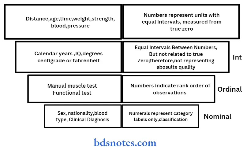
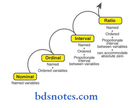
• In statistics and quantitative research methodology, various attempts have been made to classify variables (or types of data) and thereby develop a taxonomy of levels of measurement or scales of measure.
• Perhaps the best known are those developed by the psychologist Stanley Smith Stevens.
• He proposed four types: nominal, ordinal, interval, and ratio.

Scales of Measurements Definition:

• Measurements are the process of assigning numbers to variables. Measurements, as used in research, imply the qualification of information which is the assigning of some types of numbers to data.

Levels Of Measurement:

• The level of measurement describes the relationship among these three values.

Ordinal measurements:

• It involves the sorting of objects on the basis of their relative standing to each other on a specified attribute.

Interval measurement:

• It indicates not only the rank ordering of objects on an attribute but also the amount of distance between each object. Distance between numeric values on the interval scale represents an equivalent distance in the attribute being measured.

Nominal measurements:

• Are distinguished interval measurements by virtue of having a rational zero point. Most sophisticated statistical procedures require measures on the interval or ratio scales.

Ratio measurement

• There is always an absolute zero that is meaningful. This means that you can construct a meaningful fraction (or ratio) with a ratio variable. Weight is a ratio variable.

Functions Of Measurement:

1. Measurements are widely used for
2. Selection of personnel in industry/institution.
3. Various types of classification effectively.
4. In order to compare two individuals.
5. In research, It is a basic part of the research.
6. Improving classroom instruction.

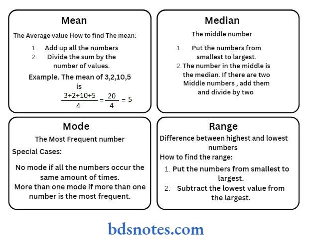
Question 6. Measurement of central tendency.
Answer:

• Measures of central tendency are used to describe what is normal for a set of data. Mean, median, and mode are the three measures of central tendency.
• The mode can be used with both numerical and nominal data The term central tendency refers to the “middle” value or perhaps a typical value of the data and is measured using the mean, median, or mode.
• Each of these measures is calculated differently, and the one that is best to use depends upon the situation.
• The central tendency is otherwise called statistical averages. The word “average” implies a value in the distribution, around which the other values are distributed.

 

Measurement of central tendency Definition:

• Central tendency is defined as “the statistical measure that identifies a single value as representative of an entire distribution.”
• Central tendency aims to provide an accurate description of the entire data. It is the single value that is most typical/representative of the collected data

Meaning Of Central Tendency:

1. A measure of central tendency is a single value that attempts to describe a set of data by identifying the central position within that set of data.
2. Measures of central tendency are sometimes called measures of central location.
3. They are also classed as summary statistics.
4. The mean (often called the average) is most likely the measure of central tendency that you are most familiar with, but there are others, such as the median and the mode.
5. The mean, median, and mode are all valid measures of central tendency, but under different conditions, some measures of central tendency become more appropriate to use than others.

Scales of Measurements Characteristics:

1. The important characteristics of an ideal measure of central tendency are
2. It should be based on all the observations of the series.
3. It should be easy to calculate and simple to understand.
4. It should not be affected by extreme values.
5. It should be rigidly defined.
6. It should be capable of further mathematical treatment
7. It should be least affected by the fluctuations of sampling.

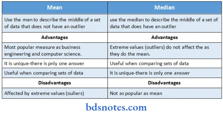
Question 7. Advantages and disadvantages of Mean, Medium.
Answer:

Question 8. Normal probability curve.
Answer:

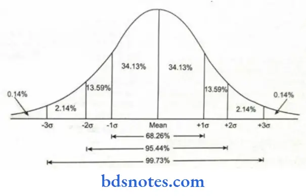
• In probability theory, the normal (or Gaussian) distribution is a very commonly occurring continuous probability distribution function that tells the probability that any real observation will fall between any two real limits or real numbers, as the curve approaches zero on either side.

Concepts Of Normal Distribution:

1. The curve is a symmetrical, bell-shaped curve with the highest frequency occurring in the middle and gradually tapering toward the extremes.
2. In a normal distribution, 68.2% of all scores cluster around the mean within approximately 1 standard deviation, 95.4% within approximately 2 standard deviations, and 99.7% within approximately 3 standard deviations.
3. It is also called a normal curve, Gauss’ curve.
4. The normal distribution (often referred to as the “bell curve” is at the core of most inferential statistics.
5. By assuming that most complex processes result in a normal distribution (we’ll see why this is reasonable), we can gauge the probability of it happening by chance.
6. To best enjoy this tutorial, it is good to come to it understanding of what probability distributions and random variables are.

Characteristics of the normal curve.

1. It will be bell-shaped.
2. It is symmetrical in distribution on either side of the mean are equal in number.
3. Its maximum height is at the mean.
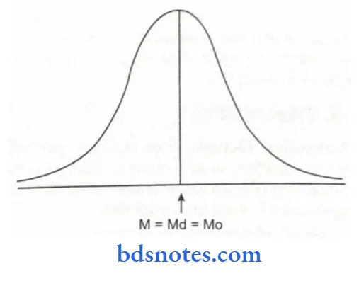
4. Mean, median and mode are coinciding.
5. It is asymptomatic (the tails never touch the baseline theoretically)
6. It has two curves – the central part is convex – when comes down, it becomes concave on both sides.
7. The normal probability curve is a continuous-type probability curve.
8. All the measures of central tendency are equal and suitable on the highest peak axis (i.e., mean = median = mode) –
9. The total area under the curve is equal to unity.
10. The normal curve has two parameters i.e., mean and standard deviation.

Importance Of Normal Probability Curve

1. The normal distribution is important is that many psychological and educational variables are distributed approximately normally.
2. Measures of reading ability, introversion, job satisfaction, and memory are among the many psychological variables approximately normally distributed. although the distributions are only approximately normal, they are usually quite close.
3. It is very helpful in forecasting. We can calculate the estimated length of the bones of animals and wood and leaves. Because if animals are one type their numbering is normally distributed.
4. The normal distribution is so important is that it is easy for mathematical statisticians to work with.
5. Normal distribution is very useful for controlling the quality of the business. With this, we can fix the limit of quality. that will be helpful for controlling the quality.
6. If we take one sample out of the universe and calculate the mean size of growing then it will normal distribution
7. This means that many kinds of statistical tests can be derived for normal distributions.
8. Almost all statistical tests discussed in this text assume normal distributions.
9. These tests work very well even if the distribution is only approximately normally
   distributed. Some tests work well even with very wide deviations from normality.
10. If the mean and standard deviation of a normal distribution are known, it is easy to convert back and forth from raw scores to percentiles.

Question 9. Type-1 and -2 Errors
Answer:

Type-1 and -1 Errors

Type-1 error occurs when the null hypothesis is rejected when it should have been accepted; also called alpha error. Type-2 error occurs when a null hypothesis is accepted when it should actually have been rejected. It is also known as beta error. These errors generally occur due to an unrepresentative sample drawn from the population.

Question 10. Level of Significance
Answer: 

• The probability of making a type-1 error is called as level of significance. It is represented by a or the p. In other words, the level of significance is the probability of rejecting the null hypothesis when it is true. In health sciences, we generally consider the level of significance either 1% (.01) or 5% (.05).
• A significance of .05 means that the researcher is willing to take the risk of being wrong 5% of the time, 5 times out of 100 when rejecting the null hypothesis.
• If the decision needs to be much more accurate, such as deciding if a nursing intervention is effective or not, the level of significance might be set at .01 or even at .001.
• With a .01 level of significance, the researcher stands the risk of being wrong 1 time out of 100 when rejecting the null hypothesis.
• At the .001 level of significance, the risk is 1 time out of 1,000. However, most of the nursing studies consider a .05 level of significance to make a decision regarding whether to accept or reject the null hypotheses.

Question 11. Descriptive And Inferential Statistics
Answer:

• Statistics is broadly classified into two categories, i.e. descriptive and inferential. Descriptive statistics deal with the enumeration, organization, and graphical representation of data.
• An example of descriptive statistics is the decennial census of India, in which all the residents are requested to provide information such as age, gender, religion, marital status, education, and occupation.
• The data obtained in such a census can be compiled and arranged into tables and graphs that describe the characteristics of the population at a given time.
• Inferential statistics provides the procedures to draw an inference about the conditions that exist in a large set of observations, i.e. an entire population from the study of a part of that set (sample). This branch of statistics is also known as sampling statistics.
• An example of inferential static is to test the efficacy of a new antihypertensive drug in which the physician will have only a limited number of hypertensive subjects on which efficacy is tested and inferences are drawn.

Descriptive Statistics:

• Descriptive statistics are used to organize and summarize data to draw meaningful interpretations.
• Descriptive statistics also allow the researcher to interpret the data meaningfully, so that research questions can be answered completely and appropriately. Descriptive statistics may be categorized in several ways; however, this chapter presents the most simplified.

Classification of the descriptive statistics that includes:

• Frequency distribution and graphical presentation (measures of condensation)
• Measures of central tendency
• Measures of dispersion
• Measures of relationship (correlation coefficient)

Question 12. Frequency Distribution
Answer:

• An appropriate presentation of data involves the organization of data in such a manner that meaningful conclusions and inferences can drawn to answer the research question. Unsorted and ungrouped records do not allow us to draw clear conclusions.
• Quantitative data are generally condensed and frequency distribution is presented through tables, charts, graphs, and diagrams.

Tables: A table presents data in a concise, systematic manner from masses of statistical data.

• Tabulation is the first step before data is used for further statistical analysis and interpretation.
• Tabulation means a systematic presentation of information contained in the data in rows and columns in accordance with some features and characteristics. Rows are horizontal and columns are vertical arrangements.

Question 13. Types and graphs in data presentation
Answer:

Graphical presentation of data:

• The main reasons for using the diagrammatic and graphic representation of data are as follows:
  • They are the most convenient and appealing ways in which statistical results may be presented.
  • They give an overall view of the entire data. They are visually more attractive than other ways of representing data.
  • It is easier to understand and memorize data through graphical representation.
  • They facilitate the comparison of data relating to different periods of time of different origins.

Types of diagrams and graphs:

• The commonly used diagrams and graphs in the presentation of data of the research studies are bar diagrams, pie diagrams, histograms, frequency polygons, line graphs, cumulative frequency curves, scattered diagrams, pictograms, and map diagrams.

Bar diagram:

• It is a convenient, graphical device that is particularly useful for displaying nominal or ordinal data. It is an easy method adopted for visual comparison of the magnitude of different frequencies.
• The length of the bars drawn vertically or horizontally indicates the frequency of a character.
• The bar charts are called vertical bar charts (or column charts) if the bars are placed vertically. When the bars are placed horizontally, we get horizontal bar charts.

There are three types of bar diagrams:

1. Simple bar diagram
2. Multiple bar diagram
3. Proportion bar diagram.

Pie diagram/sector diagram: It is another useful pictorial device for presenting discrete data of qualitative characteristics such as age groups, genders, and occupational groups in a population.

• The total area of the circle represents the entire data under consideration. Researchers must remember that only percentage data must be used to prepare pie diagrams.
• It gives comparative differences at a glance. size of each angle is calculated by multiple class percentages with a 360 or a formula may be used that.

Histogram: It is the most commonly used graphical representation of grouped frequency distribution. Variable characters of the different groups are indicated on the horizontal line (x-axis) and frequencies (number of observations) are indicated on the vertical line (y-axis).

• The frequency of each group forms a column or rectangle. Such a diagram is called a ‘histogram’.
• The area of a rectangle is proportional to the frequency of the correspondence class interval, and the total area of the histogram is proportional to the total frequency of all the class intervals.

A histogram may be drawn by using the following steps:

• Set of vertical bars the areas of which are proportional to frequencies represented.
• The difference between a histogram and from bar diagram is that a bar diagram is one-dimensional and only the length of the bar has its significance while in histograms both length and width matter.
• When class intervals are equal, frequency is taken on the y-axis, the variables on the x-axis, and adjacent rectangles are constructed.
• When the class intervals are unequal, a correction for unequal class intervals must be made.

Frequency polygon:

• It is the curve obtained by joining the midpoints of the tops of the rectangles Points of the line drawn are joined to the horizontal axis at the midpoint of the empty class-intervals histogram by straight lines. It gives a polygon, i.e. figure with many angles.
• In this, the two end data patterns are clearer than histograms. On the same axis, one can plot frequency polygons of both ends of the frequency distribution. Frequency polygons are simple and sketch an outline of Several distributions, thereby making comparisons possible.

A histogram can be drawn by using the following steps:

• Draw the histogram of the given data.
• Join the midpoints of the upper horizontal sides of each rectangle with the adjacent one by a straight line.
• Close the polygon at both ends of the distribution by extending them to the baseline.
• Hypothetical classes at each end would have to be included at each end with a frequency of zero.

Line graphs:

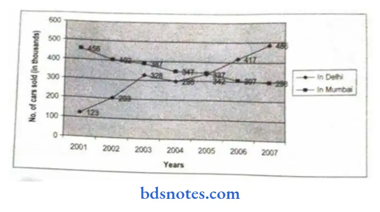
• In this, variables in the frequency polygon are depicted by line. It is mostly used where data is collected over a long period of time. On the x-axis, values of independent variables are taken and values of dependent variables are taken on the y-axis.
• The vertical axis may not start from zero, but at some point, from where frequency starts. With reference to the x- and y-axis, the given data may be plotted and these consecutive points or data are then joined by a straight line.

Cumulative frequency curve or ogive:

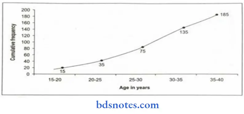
• This graph represents the data of a cumulative frequency distribution.
• For drawing an ogive, an ordinary frequency distribution table is converted into a cumulative Frequency table.
• The cumulative frequencies are then plotted corresponding to the upper limits of the classes.
• The points corresponding to cumulative frequency at each upper limit of the classes are joined by a free-hand curve. The diagram made is called ogive.

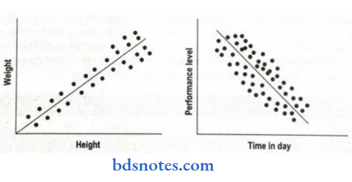
• Scattered or dotted diagrams: It is a graphic presentation that shows the nature of the correlation between two variable characters x and y on similar features or characteristics, e.g. height and weight 20 years old. Therefore, it is also called a correlation diagram.
• An example of a scattered or doctored gram is presented in

Pictograms or picture diagrams:

• This method is used to impress the frequency of the occurrence of events to common people, such as attacks, deaths, number of operations, admissions, accidents, and discharges in a population.

Map diagram or spot map:

• These maps are prepared to show the geographical distribution of frequencies of characteristics.

Limitations of graphs:

1. Confusing (may be false or true).
2. Present only quantitative aspect.
3. Get information only on one aspect or on limited characteristics.
4. They can present only approximate values.

Question 14. Degree of Freedom
Answer: 

• The interpretation of a statistical test depends on the degree of freedom. It is denoted by the abbreviation ’df‘ and a number (e.g. df=3).
• The degree of freedom indicates the number of values that are free to vary. Although the degree of freedom indicates the number of values that can vary, the concern is really focused on the number of values that are not free to vary.
• The procedure to calculate the degree of freedom varies from test to test; further details are discussed with individual tests of significance, and can be referred from there.

Question 15. Tests of Significance
Answer:

• There are several parametric (t-test, Z-test, ANOVA) and nonparametric tests (chi-square test, median test, McNemar test, Mann-Whitney Test, Wilcoxon Test, Fisher’s exact test) available to establish the statistical significance.

Parametric tests:

• These tests are also known as normal distribution statistical tests. The statistical methods of inference make certain assumptions about the populations from which the samples are drawn.
• For example, the assumptions may be that the populations are normally distributed, have the same variance, etc.; population values, as we have seen, are known as parameters; the statistical techniques that make assumptions about the parameters are called parametric techniques

Nonparametric tests:

• Researchers in the field of health sciences many times may not be aware of the nature of the distribution or other required population parameters.
• In addition, the sample may be too small to test the hypotheses and generalize the findings for the population from which the sample is drawn.
• Furthermore, many times in the observations presented in numerical figures, the scale of measurements may not be really numerical, such as grading bedsores, or ranks given to analgesic drug’s effectiveness in cancer pain management.
• In these situations, parametric tests may not be suitable, and a researcher may need different types of tests to draw inferences; those tests are known as nonparametric tests.

Question 16. Analysis of Variance (ANOVA) Test
Answer:

• When a researcher wants to compare the difference between more than two samples means; t-test I will be useful and a need for an alternative test will be felt. This need can be fulfilled by a test known as the analysis of variance (ANOVA) test.
• Therefore, it is clear that ANOVA is used to compare the more than two sample means drawn from the corresponding normal population.
• For example, a researcher wants to examine the difference in the effect of ginger on three different conditions such as nausea, vomiting, and retching, here t-test can be applied to examine the difference in the mean scores, because there are more than two groups; therefore, ANOVA will be used in this case.

Steps of application of ANOVA:

Calculate the total submissions of all the groups of observations. Calculate the sum squares of all the observations.

Calculate the total sum of squares by using the following formula;

= \(=\Sigma X^2-\frac{(\Sigma X)^2}{N}\)

Calculate the sum of squares between the groups by using the following formula.

= \(=\frac{\left(\sum \bar{X}_1\right)^2}{n_1}+\frac{\left(\sum \bar{X}_2\right)^2}{n_1}+\frac{\left(\sum \bar{X}_3\right)^2}{n_3}+\frac{\left(\sum \bar{X}_4\right)^2}{n_4}+\cdots \cdot \text { so on }-\frac{\left(\sum \bar{X}\right)^2}{N}\)

Calculate the sum of squares within the groups (error sum of squares) by using the following formula:

• = Total sum of squares – sum of squares between the groups
• Calculate the degree of freedom between and within the groups.
• df for between the groups = number of groups – 1
• df for within the groups = number of subjects in all the groups – number of groups
• df total is = number of subjects in all the groups – 1.

Calculate the mean of the sum of squares by using the following formula:

• Mean of sum of square between the groups = \(\frac{Sum of squares between the groups}{df for between the groups}\)
• Mean of sum of squares within the groups = \(\frac{Sum of squares within the groups}{df for within the groups}\)

Finally compute the F-ratio by using the following formula:

• F-ratio of square = Mean of the sum of squares between the groups
• Mean of the sum of squares within the groups the tabulated ’F” value for horizontal (df of between the groups) and vertical df (of within the groups) at the specified level of significance such as .05, 01, etc.
• If the calculated ‘F’ value is more than the tabulated ‘F’ value, then we reject the null hypothesis. If the calculated ‘F” value is less than the tabulated ’F‘ value, then we accept the null hypothesis.
• ’If the F‘ value is less than the tabulated ’F’ value, then we accept the null hypothesis.

Question 17. Vancouver style of reference.
Answer:

• Vancouver style. Vancouver is a numbered referencing style commonly used in medicine and science and consists of Citations to someone else’s work in the text, indicated by the use of a number.

Vancouver is a numbered referencing style commonly used in medicine and science, and consists of:

• Citations to someone else’s work in the text, indicated by the use of a number
• A sequentially numbered reference list at the end of the document providing full details of the corresponding in-text reference
• It follows rules established by the International Committee of Medical Journal Editors, now maintained by the U.S. National Library of Medicine.
• It is also known as Uniform Requirements for Manuscripts submitted to Biomedical Journals.
• Before using this guide check with your faculty, school, or department for their specific referencing guidelines

In-text citations:

• Insert an in-text citation:
  • when your work has been influenced by someone else’s work, for example:
    • When you directly quote someone else’s work
    • When you paraphrase someone else’s work
• General rules of in-text citation:
  • A number is allocated to a source in the order in which it is cited in the text. If the source is referred to again, the same number is used.
  • Use Arabic numerals (1,2,3,4,5,6,7,8,9)
  • Either square or curved brackets () can be used as long as it is consistent. Please check with your faculty/lecturer to see if they have a preference. For consistency in this guide, we have chosen to use round brackets for our examples
  • Superscripts can also be used rather than brackets eg….was discovered.
  • Reference numbers should be inserted to the left or inside of colons and semi-colons.
  • Reference numbers are generally placed outside or after full stops and commas – however, check with your faculty/journal publisher to determine their preference. For consistency in this guide, we are placing reference numbers after full stops.
  • Whatever format is chosen, it is important that the punctuation is consistently applied to the whole document.

Multiple works by the same author:

Each individual work by the same author, even if it is published in the same year, has its own reference number.

Citing secondary sources:

• A secondary source, or indirect citation, occurs when the ideas of one author are published in another author’s work, and you have not accessed or read the original piece of work.
• Cite the author of the work you have read and also include this source in your reference list.

In-text citation examples:

• The in-text citation is placed immediately after the text which refers to the source being cited

Using round brackets:

• As one author has put it “The darkest days were still ahead”.

Using square brackets:

• As one author has put it “the darkest days were still ahead”.

Using superscript:

• As one author has put it “the darkest days were still ahead”.
• The author’s name can also be integrated into the text
• Scholtz has argued that

Including page numbers with in-text citations:

• Page numbers are not usually included with the citation number. However, should you wish to specify the page number of the source the page/s should be included in the following format:
• As one author has put it “The darkest days were still ahead”,
• As one author has put it “the darkest days were still ahead”.
• Scholtz (1 p16-18) has argued that

Citing more than one reference at a time:

• The preferred method is to list each reference number separated by a comma, or by a dash for a sequence of consecutive numbers. There should be no spaces between commas or dashes

For example: (1,5,6-8)

Reference List:

• References are listed in numerical order, and in the same order in which they are cited in text. The reference list appears at the end of the paper.
• Begin your reference list on a new page and title it ‘References.”
• The reference list should include all and only those references you have cited in the text. (However, do not include unpublished items such as correspondence).
• Use Arabic numerals (1, 2, 3, 4, 5, 6, 7,8,9).
• Abbreviate journal titles in the style used in the NLM Catalog
• Check the reference details against the actual source indicating that you have read a source when you cite it.